Nominal variables are more than just a name

Nominal variables are a type of categorical variables that take different values for which the order does not matter. They are variables that help to differentiate some elements from others by their qualities and not by their quantity or their degree of possession of a certain modality.

Some examples of classic nominal variables in clinical trials are the randomization group, sex, diagnosis, type of treatment, hospital where the patients were recruited, whether a certain medical test was performed, type of adverse event, etc. Other nominal variables can be any identifying variable, for example: person’s full name, ID card number, order number, telephone number, medical history number, etc.

First, describing…

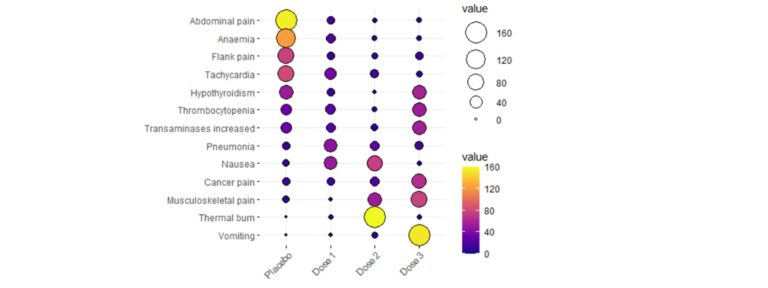
The nominal variables descriptive analysis usually begins with the study of the distribution of the number of cases in each category and their percentages. Additionally, it is essential to represent them graphically in a clear way. You can use classic graphs, such as the bar chart or pie chart, but if you want to represent multiple variables simultaneously in a very visual way, some examples are given below:

Association between nominal variables – Why can be friends?

The analysis to study the relationship between two nominal variables is often based on the study of the chi-square coefficient. It is one of the best known and widely used analyses in any scientific discipline. This analysis is based on several assumptions, but one of the most important is associated with the expected joint frequencies, according to which no more than 20% of the cells should have an expected frequency of less than 5 cases. When this assumption is not met, the test loses power. When analyzing correlations with this coefficient, a number of nuances must be taken into account:

• If the table is a 2×2 table, the Yates’ correction for continuity should be used.
• If the sample size is very small –less than 30 cases– and a 2×2 table is available, Fisher’s exact test should be used.

Since the chi-square coefficient is not bounded (its value ranges from 0 to infinity), it is not possible to study the strength of the correlation, although residual analyses allow us to study the concentration of cases in the cells of the contingency table.

There are other coefficients that make it possible to study the strenght of the association between two nominal variables:

If nominal variables change over time… follow them closely!

If you have a nominal variable measured over multiple time periods and you want to study whether there are changes in the distribution of its modalities, there are a series of techniques that allow you to study whether there are significant variations:

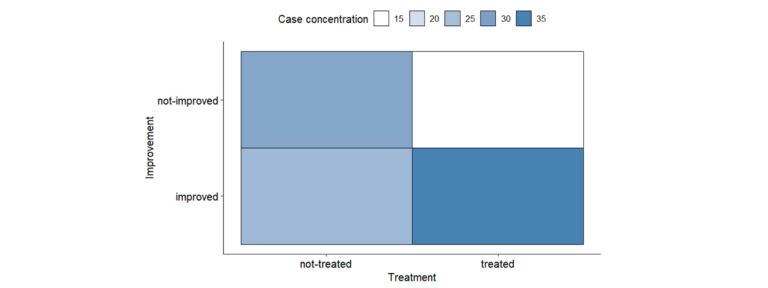
A word about odds ratios and the Relative Risk Ratio

In order to understand the concept of odds ratio, it is necessary to understand the following concepts associated with it:

• Probability: it is a measure of how likely it is that a phenomenon or event will occur. This value ranges from 0 to 1, with 0 meaning that the event cannot happen and 1 meaning that the event is certain to occur. For example, if the probability of improvement is 0.60, the probability of no improvement would be 0.40.
• Odds: it is the probability of an event happening divided by the probability of it not happening.

Odds range from 0 to infinity and can be calculated for the occurrence of the event as well as for the non-occurrence of the event. In the example, there would be two odds: the odds of improvement would be 0.60/0.40=1.5 and the odds of no improvement would be 0.40/0.60=0.667. These are interpreted as ratios, i.e., the number of times something can happen over the number of times it cannot happen. In this case, the patient is more likely to improve.

Odds ratios (OR) are the quotient between the two odds and also range from 0 to infinity, but how is an OR interpreted in a basic way?

• When the OR is 1, it indicates there is no association between the variables.
• Values below 1 indicate a negative association between the variables and values greater than 1 indicate a positive association between the variables.
• The further the OR is from 1, the stronger the relationship.

In the case of the Relative Risk Ratio, it is defined as the quotient of the odds of having the disease or presenting the outcome of interest if the predictive factor –i.e., the risk factor– is present or absent.

To interpret relative risk, let us consider an RR of 2. This result means that the risk in one group is twice as high as in the other group. If it is equal to 1, it is equal for both groups and if it is less than 1, the risk is higher for the other group.

The main difference with the OR is that the Relative Risk Ratio is used primarily in the assessment of prospective studies, while the OR is used primarily in the analysis of retrospective studies.

Can anything else be done with nominal variables?

Of course! The analysis of nominal variables can go beyond studying their descriptive behavior and their bivariate relationship. Some examples of possible analyses are:

• Log-linear models: if you want to analyze the relationship between three or more nominal variables.
• Classification machine learning algorithms: if you want, for example, to predict the probability of a patient recovering (or not) based on a series of clinical variables, these algorithms are very useful.
• Text analysis and open-ended responses: analyses linked to Natural Language Processing are used for text analysis, for example, of open-ended responses given during an interview with patients to determine their health status.

Mercedes Ovejero and Jaime Ballesteros

Biostatistics Unit of Sermes CRO

• By Sermes CRO
• 13/04/2023
• Nominal variables